1 - A first minimal case
Compute tree light interception by symmetric crowns in an axis-aligned rectangle plot
Source:vignettes/web_only/1-minimal_case.Rmd
1-minimal_case.RmdIntroduction
This is the first tutorial, showing you how to solve a basic problem using the SamsaRaLight package on a ‘marteloscope’ plot — a basic format for applying the package. A ‘marteloscope’ is a plot used for harvesting exercises in the field. Trees are inventoried inside a delimited plot, which is generally 1 ha (100 m x 100 m) squared.
We will demonstrate this using the Prenovel dataset, which is stored
in the package as SamsaRaLight::data_prenovel. This dataset
represents an uneven-aged stand of fir, spruce and beech located in the
Jura mountains in France. Further information can be found in the data
documentation.
The next tutorials explain how to create a virtual stand from a more complex tree inventory (4 - Create a virtual stand from a more complex tree inventory).
Input data
Format the tree inventory
First, the user needs to define the individual trees composing the
stand with their crown dimensions. The data frame must be created with a
specific format and variables. See documentation using
?SamsaRaLight::check_inventory() to understand the format
of the trees dataset, and validate it using the same function.
The dataframe must contain mandatory information about the trees: a
unique integer id (id_tree), the species name
(species), coordinates in meters (x,
y) and diameter at breast height in cm
(dbh_cm). The x and y coordinates
must be given in meters on a flat plane (not considering slope), and the
z coordinate will be computed automatically during the
process from stand geometry. Be careful, you cannot use
longitude/latitude (WGS84 coordinates system), as it is angular
coordinates, thus not representing correctly relative distance between
each tree. Consider converting the coordinates in a planar reference
system such as local UTM. We will see further in the next tutorials that
the SamsaRaLight package can automatically manage lon/lat coordinates,
typically for trees inventoried with GPS data giving long/lat
coordinates (4 - Create a virtual stand from more complex tree
inventory).
In this tutorial, we represent the tree crowns with simple shapes,
defined in the crown_type column by a specific code: “E”
(for an ellipsoid) or “P” (for a paraboloid). The ellipsoidal shape “E”
is commonly used for broadleaved species, whereas a paraboloidal shape
“P” is commonly used for conifers. When using simple crown shapes, the
user must provide only 3 values to define the crown dimensions: the
height of the tree (h_m in meters), the height of the base
of the crown (hbase_m in meters) and the crown maximum
radius that is the same is the four cardinal directions as we consider
simple symmetric crowns (rn_m for north, re_m
for east, rs_m for south and rw_m for west,
all in meters). When considering those type of simple crown shapes (“E”
or “P”), the user must not provide the hmax_m variable,
which is the height at which the crown radius is maximum. Indeed, it is
automatically computed during the process, being set to the crown base
height
()
when considering a paraboloidal shape “P”, and set at the middle of the
crown for an ellipsoidal shape “E”
().
input_trees_inv <- SamsaRaLight::data_prenovel$trees
head(input_trees_inv)
#>   id_tree    species       x       y  dbh_cm crown_type     h_m hbase_m hmax_m
#> 1       1 Abies alba 77.7336 71.0808 22.9320          P 14.8120  3.3073     NA
#> 2       2 Abies alba 62.5783 65.1864 18.2397          P 12.9612  4.7429     NA
#> 3       3 Abies alba 84.0060 95.2483 22.8472          P 15.8187  4.9055     NA
#> 4       4 Abies alba 58.9521 97.9011 19.1539          P 11.7033  4.2050     NA
#> 5       5 Abies alba 33.3423 39.4053 19.8852          P 14.6597  3.8346     NA
#> 6       6 Abies alba 57.5743  2.0656 20.1293          P 16.6530  7.6860     NA
#>     rn_m   re_m   rs_m   rw_m crown_lad
#> 1 3.0204 3.0204 3.0204 3.0204     0.767
#> 2 3.0896 3.0896 3.0896 3.0896     0.767
#> 3 2.8350 2.8350 2.8350 2.8350     0.767
#> 4 2.5196 2.5196 2.5196 2.5196     0.767
#> 5 2.8208 2.8208 2.8208 2.8208     0.767
#> 6 3.2436 3.2436 3.2436 3.2436     0.767

# Check the format of the inventory table
SamsaRaLight::check_inventory(input_trees_inv)
#> Inventory table successfully validated.
The user can observe its validated inventory using the function
SamsaRaLight::plot_inventory().
plot_inventory(input_trees_inv)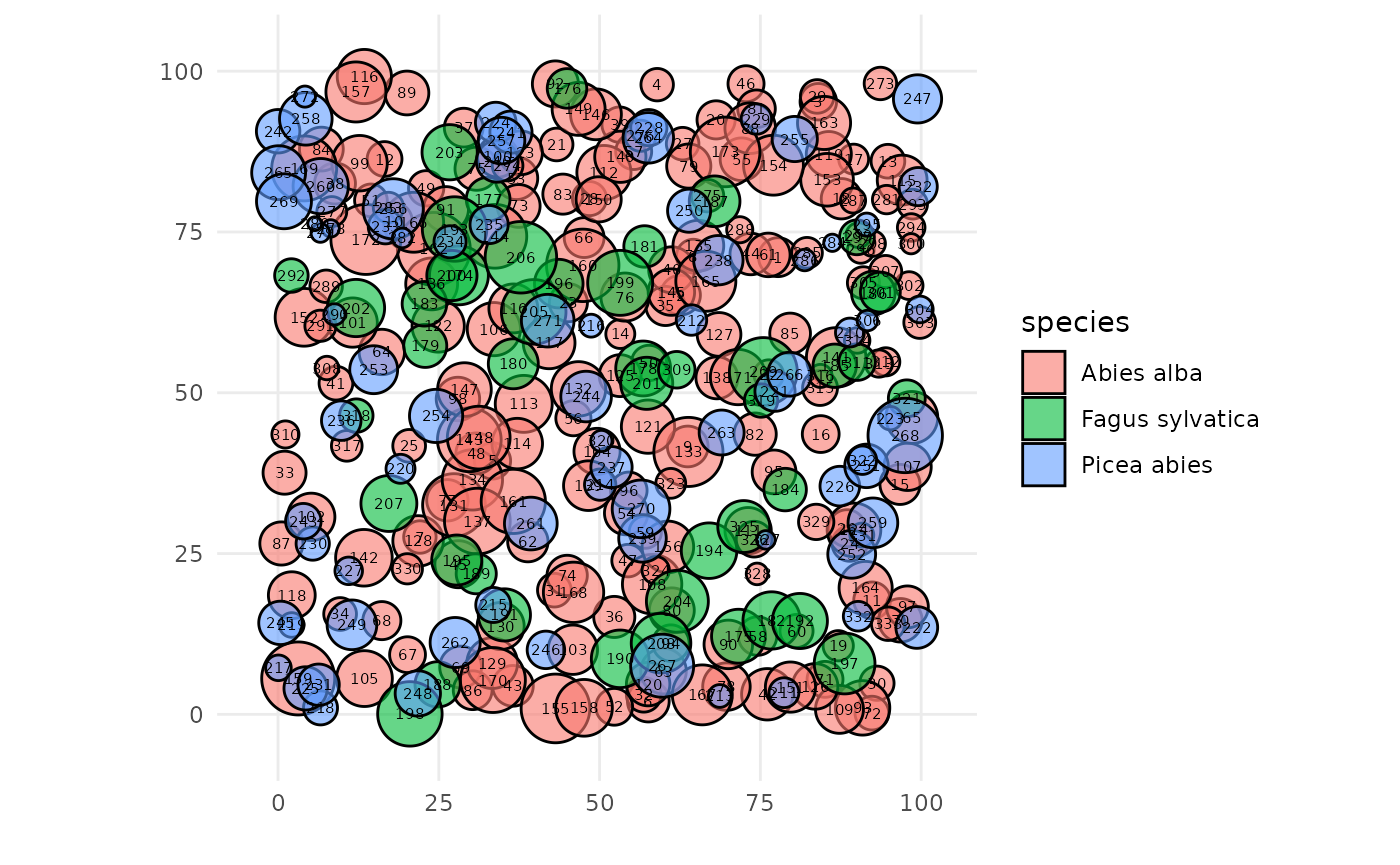
In the next tutorials, we will explain more in details the column
crown_lad, set by default to a value of 0.5 for each tree
(3 - Understand the transmission model) and consider more complex,
asymmetric crown shapes (5 - Represent the crowns with more complex
shapes).
Create the SamsaRaLight input stand
The SamsaraLight ray-tracing model needs to be run on a axis-aligned rectangle stand that is split into square cells, with a given homogeneous slope, orientation and aspect. Moreover, the user needs to precise the plot latitude (Y-axis in WGS84 in degrees) as the model considers that light rays’ geometry vary with plot latitude, discussed further in the Tutorial 2 (2 - Understand ray-tracing).
The package provides a function that creates a standardized
SamsaRaLight virtual stand as a sl_stand R S3 object:
SamsaRaLight::create_sl_stand(). This function needs 5
mandatory arguments: the tree inventory table (tree_inv,
formatted as described above), the size of the square cell that split
the rectangle SamsaRaLight stand (cell_size in meters), the
plot latitude (latitude) and three variables defining the
plane stand geometry (slope, aspect and
north2x, all in degrees). The function checks internally
that all arguments are correct and well formatted (set the argument
verbose = FALSE to avoid success messages).
Optionally but essential here to well define your virtual stand from
the tree inventory, the user can define the inventory zone with the
argument core_polygon_df. The polygon is defined by a
data.frame that contains the coordinates x and
y of the vertices of the zone where the trees have been
inventoried. The tutorial 4 (4 - Complex inventories) will address both
the automatic computation and modification of the inventory zone.
The cell_size argument defines the precision of the
SamsaRaLight ray-tracing model. The ray-tracing model will casts rays
towards the center of each cell and estimate the light arriving to this
cell after attenuation by tree crowns. The smaller the cells are
defined, the more rays the model casts per m2. The default
cell_size value is 5, leading to a good compromise between
fast computation time and sufficient model precision for output
variables. The user can go towards the maximum precision which is 1
(1m*1m square cells) to produce high-resolution shading maps (see the
end of this tutorial), but will lead to much heavier computation time
and memory use. Indeed, computation time is not proportional to
cell_size but rather quadratic: the number of cells in the
plot increases quadratically with the cell size, and also consequently
is the total number of cast rays during the simulation (which is the
main factor for computation time and memory use).
The north2x argument is the angle from real North to the
virtual plot X-axis (clockwise), allowing to convert the system from
geographic (tree inventory) to mathematics (SamsaRaLight simulation).
The default 90° corresponds to a Y-axis oriented toward true North (0°:
x-axis points North, 90° : x-axis points East, 180° : x-axis points
South, 270° : x-axis points West).
The slope and aspect arguments define the
geometry in case of a non-plane stand, with the aspect variable
representing the direction the slope faces downhill, defined by the
angle of the steepest downslope direction measured clockwise from true
North (0°: North-facing slope, 90°: East-facing slope, 180°:
South-facing slope, 270°: West-facing slope). The Tutorial 2 (2 -
Understand ray-tracing) also shows how the light on the ground varies
with stand geometry.
input_sl_stand <- SamsaRaLight::create_sl_stand(

  # Tree inventory formatted table
  trees_inv = input_trees_inv,

  # Precision of the SamsaRaLight model
  cell_size = 1,

  # Stand information
  latitude = SamsaRaLight::data_prenovel$info$latitude,
  slope = SamsaRaLight::data_prenovel$info$slope,
  aspect = SamsaRaLight::data_prenovel$info$aspect,
  north2x = SamsaRaLight::data_prenovel$info$north2x,

  # Definition of the inventory zone definition
  core_polygon_df = SamsaRaLight::data_prenovel$core_polygon
)
#> SamsaRaLight stand successfully created.
The user can observe the creating SamsaRaLight virtual stand object
(sl_stand S3 object) using the base functions
print(), summary() and plot().
The plot() function allows to observe the stand in two
views: a stand map with circles representing the located maximum crown
radius of trees from above, or a top-down plot mainly showing heights of
crowns and trunks from a South-view (facing North) and a East-view
(facing West). Computation time can be long for the stand map as the
trees are plotted in order of tree height to well represent the vertical
structure of the stand.
print(input_sl_stand)
#> SamsaRaLight stand of 1 ha with 333 trees and 0 sensors (100 x 100 cells, 1 m)
summary(input_sl_stand)
#>
#> SamsaRaLight stand summary
#> ================================
#>
#>
#> Inventory (core polygon):
#>   Area              : 1.00 ha
#>   Trees             : 333
#>   Density           : 333.0 trees/ha
#>   Basal area        : 35.41 m2/ha
#>   Quadratic mean DBH: 36.8 cm
#>
#> Simulation stand (core + filled buffer):
#>   Area              : 1.00 ha
#>   Trees             : 333
#>   Density           : 333.0 trees/ha
#>   Basal area        : 35.41 m2/ha
#>   Quadratic mean DBH: 36.8 cm
#>
#> Stand geometry:
#>   Grid              : 100 x 100 (10000 cells)
#>   Cell size         : 1.00 m
#>   Slope             : 6.00 deg
#>   Aspect            : 144.00 deg
#>   North to X-axis   : 54.00 deg
#>
#> Number of sensors: 0
plot(input_sl_stand)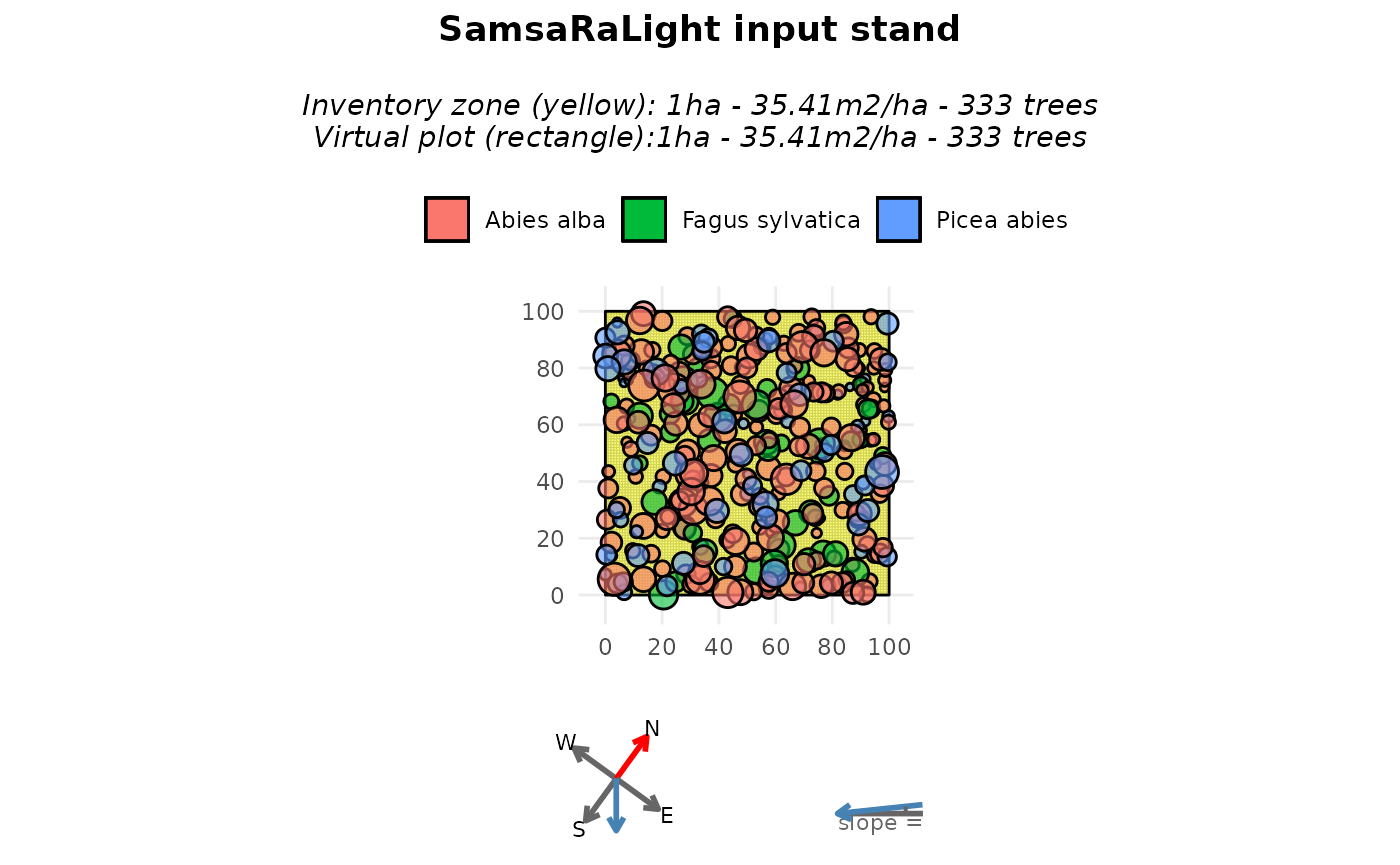
plot(input_sl_stand, top_down = TRUE)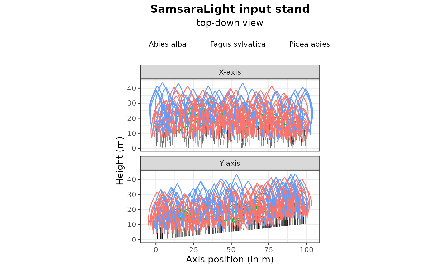
These functions are essential for assessing the consistency of the input inventory data and its conversion into a SamsaRaLight stand. They act as a preliminary diagnostic to ensure, for example, that no trees are forgotten (see the stand summary), the trees are correctly positioned within the virtual stand (see the stand map), that the north2x and aspect variables are correctly defined according to the tree inventory (see the plotted compass next to the stand map, with the blue dotted arrow showing the downslope direction), and that the crown dimensions are consistent (see the top-down view).
Monthly radiations
Then, the user needs to define in a data frame the monthly energy specific to its plot location. For each month (represented by an integer number between 1 and 12), one needs to inform as the global monthly energies (in ), and as the ratio of diffuse energy relative to global energy (needed to represent the proportion of diffuse and direct energy). The discretization of diffuse and direct rays from the given radiation dataset is discussed in the next tutorial (2 - Understand ray-tracing).
This data frame can be automatically constructed using the
SamsaRaLight function
SamsaRaLight::get_monthly_radiations(), given the latitude
and longitude of the plot. It gets radiation data from the PVGIS
European database but needs an Internet connection. Otherwise, the
monthly radiation data frame used in this tutorial (Prenovel stand) is
stored within the package and can be retrieved using
SamsaRaLight::data_prenovel$radiations.
# Get the monthly radiation data frame
input_monthly_radiations <- SamsaRaLight::get_monthly_radiations(
  SamsaRaLight::data_prenovel$info$latitude,
  SamsaRaLight::data_prenovel$info$longitude
)

input_monthly_radiations
#>    month     Hrad  DGratio
#> 1      1 137.0902 0.580625
#> 2      2 206.3025 0.506875
#> 3      3 353.8260 0.493125
#> 4      4 465.8220 0.490000
#> 5      5 535.2458 0.508750
#> 6      6 618.1785 0.463750
#> 7      7 655.1730 0.425000
#> 8      8 557.6332 0.436250
#> 9      9 423.9382 0.446875
#> 10    10 280.2780 0.475000
#> 11    11 157.9635 0.538750
#> 12    12 116.4960 0.587500

# Check that it the format is correct
check_monthly_radiations(input_monthly_radiations)
#> Radiation table successfully validated.
Run SamsaRaLight
From now, you can easily run the SamsaraLight ray-tracing model using
the function run_sl() from the only two mandatory
arguments: the created SamsaRaLight virtual stand object
sl_stand and the monthly radiations table
monthly_radiations.
The package SamsaRaLight allows for running the simulation in
parallel setting the argument parallel_mode = TRUE. When
activating the parallel_mode, the simulation will take by default all
the internal threads that are avaikable, but the user can decide how
many cores to dedicate to the simulation with the argument
n_threads. During the simulation, a message will appear to
specify to the user how many cores are used by the simulation, and how
many are available with the device, but the user can silence those
messages with verbose = TRUE argument. The parallelisation
is done internally across independent cells, while running sequentially
each ray for a given cell. By doing so, the parallel mode is even
essential when the number of cells is large. Parallelisation is done
using OpenMP, but on platforms or compilers that do not support OpenMP,
parallelisation is disabled and computations run in sequential mode
(i.e. parallel_mode = FALSE).
sl_output <- SamsaRaLight::run_sl(

    # Mandatory arguments
    sl_stand = input_sl_stand,
    monthly_radiations = input_monthly_radiations,

    # Parallelisation arguments
    parallel_mode = TRUE,
    n_threads = NULL
  )
#> Warning in sl_set_openmp(parallel_mode = parallel_mode, num_threads =
#> as.integer(n_threads), : OpenMP not available: running sequentially.
#> parallel mode disabled because OpenMP was not available
#> SamsaRaLight simulation was run successfully.
For advanced users, another function is available
SamsaRaLight::run_sl_advanced(), allowing to control deeper
ray-tracing parameters. The user-friendly function
SamsaRaLight::run_sl() internally wrap the advanced version
with default parameters. In the tutorials, we will not adress this
advanced function, but all parameters with default values can be find
following the documentation of this function. Otherwise, feel free to
contact the main authors for a deeper use of the package and the
model.
Simulation output
The output is a complex S3 R object, with first a list of two
elements: $input (that gathers inputs of the model defined
above $input$sl_stand and
$input$monthly_radiations, associated to the parameters of
the simulation $input$params) and $output that
essentially contains output light variables at the tree-level
output$light$trees and at the cell-level
output$light$cells. You can also observe
output$light$sensors that are the light output at a located
virtual light sensor, but this is discussed in the Tutorial 6 (6 - Add
virtual sensors on the ground). Optionnaly, the user can set the
run_sl() function argument detailed_output to
TRUE in order to have more information about the rays discretisation and
interceptions, but it is also discussed further in the next tutorial (2
- Understand ray-tracing). In this tutorial, we will focus here on both
the tree- and cell-level output light variables, stored in
output$light.
The object $output$cells contains output light variables
for each cell, identified by its unique id (id_cell, linked
to the input cell dataframe sl_output$input$sl_stand$cells
to retrive cell center coordinates). There are 3 output variables, which
are e (for the energy arriving on the cell in MJ/m2),
pacl (for proportion of above light canopy, which is the
ratio between the energy arriving on the cell and the energy before
interception by the trees) and punobs (for the proportion
of energy on the cell that comes from unobstructed rays, i.e. rays that
have not been intercepted by any trees).
str(sl_output$output$light$cells)
#> 'data.frame':    10000 obs. of  4 variables:
#>  $ id_cell: int  1 2 3 4 5 6 7 8 9 10 ...
#>  $ e      : num  390 446 424 428 426 ...
#>  $ pacl   : num  0.086 0.0984 0.0935 0.0943 0.094 ...
#>  $ punobs : num  0.357 0.449 0.518 0.479 0.394 ...
The object $output$trees contains output light variables
for each trees, identified by its unique id (id_tree).
There are 4 output variables, which are e (for the total
energy intercepted by the tree in MJ), epot (for the
potential energy intercepted by the tree without considering its
neighbors in MJ, i.e. the total energy intercepted if the tree was alone
with the same crown dimensions),
(which is a light competition index and a good proxy for tree dynamics,
see Beauchamp et al. 2025, representing the real intercepted energy
compared to the potential energy it could intercept without competition)
and punobs (for the proportion of energy intercepted by the
tree that comes from unobstructed rays, i.e. rays that have not been
intercepted by any other trees).
str(sl_output$output$light$trees)
#> 'data.frame':    333 obs. of  5 variables:
#>  $ id_tree: int  116 92 46 273 176 4 272 157 89 29 ...
#>  $ epot   : num  413020 276836 225132 89770 233549 ...
#>  $ e      : num  117102 100888 58738 16553 8306 ...
#>  $ lci    : num  0.716 0.636 0.739 0.816 0.964 ...
#>  $ eunobs : num  90129 87856 49288 12039 1494 ...
The user can observe the output of the SamsaRaLight simulation object
(sl_output S3 object) using the base functions
print(), summary() and plot().
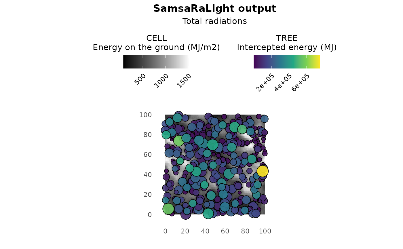
The plot() function allows to observe the stand map with
tree- and cell-level colouring depending on the output light variables.
By default, the plot shows the light competition index LCI for trees and
the relative light on the ground PACL for cells, as there are good
proxies for estimating tree and stand dynamics. In addition, the
argument show_trees can be set to FALSE to plot only a
shade map as a nice plot for representing the understorey light. Light
variables to plot can be defined independently for both trees and cells
by setting what_trees and what_cells
arguments. For example, setting what_trees = "intercepted"
and what_cells = "absolute allows to better catch the
differences in light energies between trees and cells. However, be
careful about the colours of the cells, white areas do no mean cells in
high-light but brighter cells relatively to the others, it could be
confusing without precise legend.
print(sl_output)
#> SamsaRaLight output with 10000 cells, 333 trees and 0 sensors (no detailed output)
summary(sl_output)
#>
#> SamsaRaLight simulation summary
#> ================================
#>
#> Trees (crown interception)
#> ---------------------------
#>       epot               e                 lci
#>  Min.   :  11227   Min.   :   650.7   Min.   :0.07583
#>  1st Qu.: 171380   1st Qu.: 23632.9   1st Qu.:0.58652
#>  Median : 306488   Median : 71049.0   Median :0.73860
#>  Mean   : 334326   Mean   :118512.4   Mean   :0.70663
#>  3rd Qu.: 468539   3rd Qu.:183633.1   3rd Qu.:0.85197
#>  Max.   :1044676   Max.   :750436.9   Max.   :0.99319
#>
#> Cells (ground light)
#> -------------------
#>        e                pacl             punobs
#>  Min.   :  71.51   Min.   :0.01577   Min.   :0.0000
#>  1st Qu.: 375.82   1st Qu.:0.08287   1st Qu.:0.3981
#>  Median : 559.50   Median :0.12337   Median :0.5676
#>  Mean   : 604.61   Mean   :0.13331   Mean   :0.5389
#>  3rd Qu.: 780.16   3rd Qu.:0.17202   3rd Qu.:0.7046
#>  Max.   :1525.78   Max.   :0.33643   Max.   :0.9370
#>
#> Sensors
#> -------
#> No sensor energy variables available
plot(sl_output)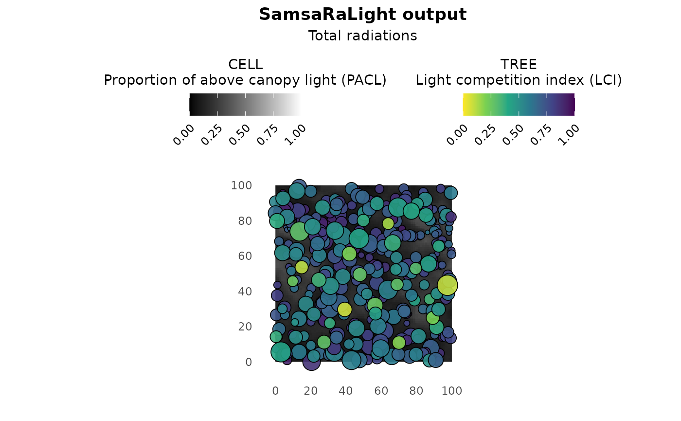
plot(sl_output, show_trees = F)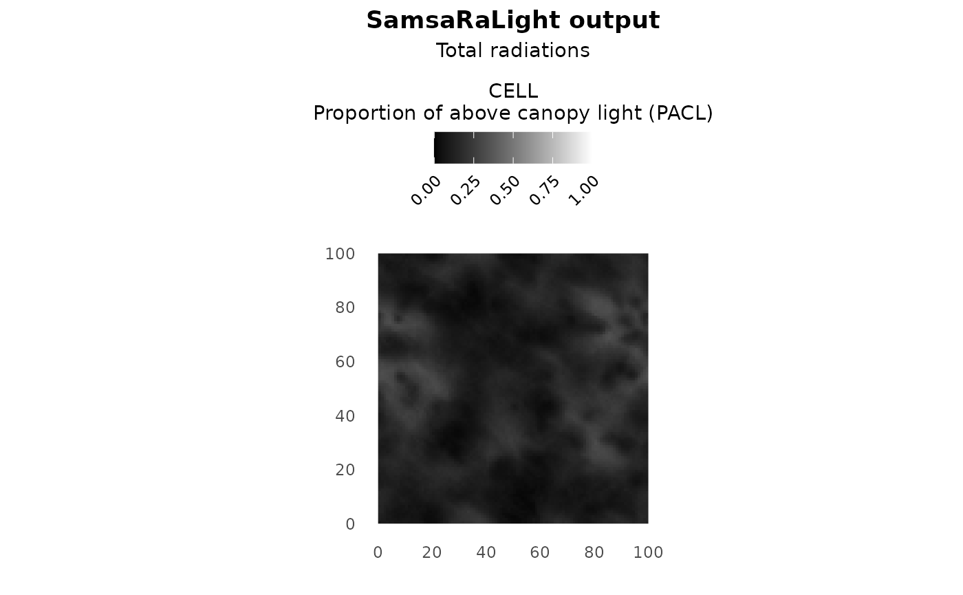
plot(sl_output, what_trees = "intercepted", what_cells = "absolute")