Asymmetric crowns in a non-axis-aligned stand • SamsaRaLight

library(SamsaRaLight)
library(dplyr)
#> 
#> Attaching package: 'dplyr'
#> The following objects are masked from 'package:stats':
#> 
#>     filter, lag
#> The following objects are masked from 'package:base':
#> 
#>     intersect, setdiff, setequal, union

Introduction

In previous tutorials, tree crowns were represented using simple symmetric shapes (“E” and “P”). However, real tree crowns are often asymmetric, both horizontally (different crown radii in different directions) and vertically (maximum crown width not located at mid-crown for “E” nor crown base height for “P”).

In this vignette, we will use an inventory with asymmetric crown shapes. We will work with a non axis-aligned rectangle inventory zone to show that rotating a stand where crown are represented as assymetric shapes is tricky.

Crown shapes available in SamsaRaLight

SamsaRaLight supports the following crown types: "E", "P", "2E", "4P", "8E". The number indicates how many crown parts are used. The letter indicates the geometric shape (Ellipsoid or Paraboloid). Choose the simplest crown type that matches your data quality.

Symmetric crown shapes

Symetric shapes used in the Tutorial 1, defined by the mean crown radius (mean of the four radius rn_m, rs_m, re_m and rw_m) and the crown depth (computed as h_m - hbase_m. These shapes are simple and efficient, but cannot represent crown asymmetry, knowing that crown asymmetry strongly affects light interception.

“E” — Symmetric ellipsoid

Single ellipsoidal volume
Same radius in all directions
Maximum radius automatically computed at mid-crown height (hmax_m = hbase_m + (h_m - hbase_m) / 2

“P” — Symmetric paraboloid

Single paraboloid volume
Same radius in all directions
Maximum radius located at crown base height (hmax_m = base_m)

Asymmetric crown shapes

More complex shapes are created by splitting the crown into multiple geometric parts.

“2E” — Vertical asymmetry

Crown split into an upper and a lower ellipsoid
Allows vertical asymmetry
Requires hmax_m, the height of maximum crown radius

Crown remains horizontally symmetric. Use this shape when crown expansion is not centered vertically.

“4P” — Horizontal asymmetry

Crown split into four horizontal paraboloids
Different radii allowed in the four cardinal directions: rn_m (north), rs_m (south), re_m (east) and rw_m (west)
Crown is vertically symmetric: hmax_m is NOT required (paraboloid, thus hmax = hbase_m)

Use this shape when crowns are laterally deformed by competition.

“8E” — Full asymmetry

Crown split into upper and lower parts (vertical asymmetry)
each split into four cardinal directions (horizontal asymmetry)
Requires: rn_m, rs_m, re_m, rw_m and hmax_m

This is the most detailed crown representation available.

Context and data

We illustrate asymmetric crowns using the Bechefa marteloscope, stored in the package as SamsaRaLight::data_bechefa.

This marteloscope was installed in Belgian Ardennes by Gauthier Ligot in the scope of the IRRES project, which investigates the transition from even-aged to uneven-aged forest management. This is a mature mixed stand of Douglas fir and spruce in the Belgian Ardennes. The stand has been uneven-aged for more than 10 years.

All trees use the "8E" crown type, allowing both horizontal and vertical asymmetry. Each tree provides four directional crown radii (rn_m for maximum crown radius pointing north, rs_m for south, re_m for east, rw_m for west) and the height of maximum crown expansion (hmax_m).

head(SamsaRaLight::data_bechefa$trees)
#>   id_tree     species     x    y    dbh_cm crown_type  h_m hbase_m hmax_m rn_m
#> 1     103       abies 163.1 67.3  68.43663         8E 38.5    16.6   28.2 4.32
#> 2     615 pseudotsuga  66.8 41.4  95.49297         8E 50.2    14.0   33.3 7.01
#> 3     102 pseudotsuga 159.2 58.2 111.72677         8E 48.2    10.8   27.1 8.38
#> 4     708 pseudotsuga  43.8 34.2 116.81973         8E 51.0    15.8   27.0 7.37
#> 5     707 pseudotsuga  51.4 34.1  99.94930         8E 50.5    16.0   26.7 6.73
#> 6     712 pseudotsuga  57.2 17.0 112.04508         8E 51.4    14.4   26.5 5.02
#>   rs_m re_m rw_m crown_lad
#> 1 4.12 3.70 5.20       0.6
#> 2 6.45 5.87 4.15       0.6
#> 3 6.72 4.69 6.51       0.6
#> 4 7.43 9.85 5.44       0.6
#> 5 5.16 3.40 5.76       0.6
#> 6 6.02 5.00 5.32       0.6

Create the stand

The subsequent steps are identical to those used with symmetric crowns (see Tutorial 1). Introducing asymmetric crowns only requires adapting the initial tree inventory. Horizontal asymmetry is clearly visible in the plots, whereas vertical asymmetry is more difficult to perceive graphically because crowns are displayed as projected shapes.

It is important to note that the north2x parameter must be a multiple of 90° (i.e. 0°, 90°, 180°, or 270°) when the virtual stand contains at least one horizontally asymmetric crown type (i.e. "4P" or "8E"). Horizontal asymmetry is defined by assigning different crown radii to the four cardinal directions (north, south, east, and west). These four directional radii are internally converted into planar X–Y axis-aligned radii according to the value of north2x.

stand_bechefa <- SamsaRaLight::create_sl_stand(
  trees_inv = SamsaRaLight::data_bechefa$trees,
  
  cell_size = 5,
  
  latitude = SamsaRaLight::data_bechefa$info$latitude,
  slope = SamsaRaLight::data_bechefa$info$slope,
  aspect = SamsaRaLight::data_bechefa$info$aspect,
  north2x = SamsaRaLight::data_bechefa$info$north2x,
  
  core_polygon_df = SamsaRaLight::data_bechefa$core_polygon
)
#> SamsaRaLight stand successfully created.

plot(stand_bechefa)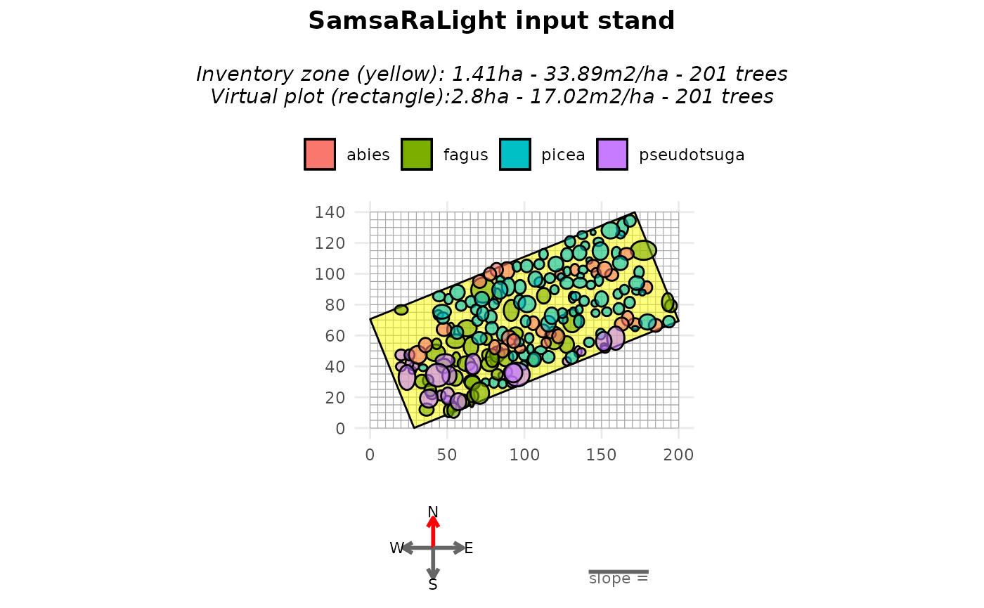

plot(stand_bechefa, top_down = TRUE)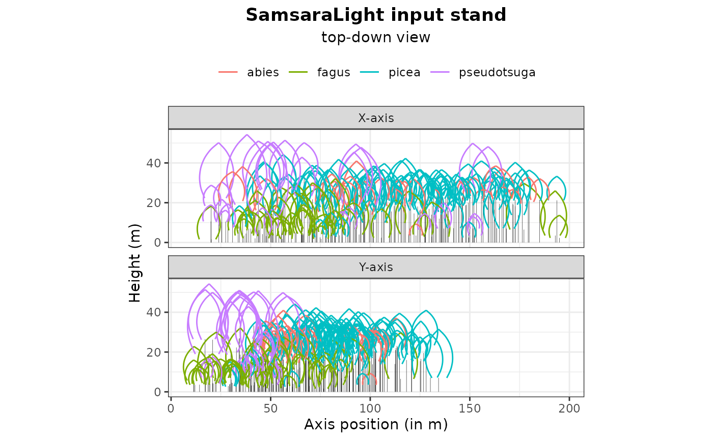

Fill around the inventory zone

Such as in the previous tutorial, we may want to rotate the stand in order to axis-align it. However, because of the same reason as the described above for north2x when considering at least one horizontal asymmetric crown, we can rotate the stand only by a multiple of 90°, leading to impossibility to axis-align the stand in most case. For this reason, the argument “modify_polygon = aarect” is desactivated if at least one horizontal asymmetric crown is present in the stand. However, the user can still transform and ensure its inventory zone is a perfect rectangle (minimum enclosing rectangle area) with the argument modify_polygon = "rect". Otherwise, to not modify the given polygon, the default argument is modify_polygon = "none".

To counteract the fact that plot is empty around the non-axis aligned rectangle inventory zone, we can use the argument fill_around = TRUE when creating the vitual stand with the create_sl_stand(). This will add virtual trees outside the inventory polygon, within the simulation grid:

sampled from the inventoried trees,
randomly positioned outside the inventory zone,
until the surrounding area reaches the same basal area per hectare as the inventory zone.

stand_bechefa_filled <- SamsaRaLight::create_sl_stand(
  trees_inv = SamsaRaLight::data_bechefa$trees,
  
  cell_size = 5,
  
  latitude = SamsaRaLight::data_bechefa$info$latitude,
  slope = SamsaRaLight::data_bechefa$info$slope,
  aspect = SamsaRaLight::data_bechefa$info$aspect,
  north2x = SamsaRaLight::data_bechefa$info$north2x,
  
  core_polygon_df = SamsaRaLight::data_bechefa$core_polygon,
  modify_polygon = "rect",
  fill_around = TRUE
)
#> SamsaRaLight stand successfully created.

plot(stand_bechefa_filled)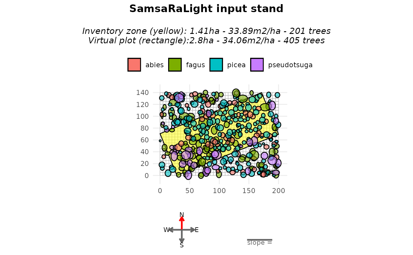

When plotting, the argument only_inv = TRUE allows displaying only the inventoried trees (inside the yellow polygon). Added trees are identified in the stand object using the logical column added_to_fill.

table(stand_bechefa_filled$trees$added_to_fill)
#> 
#> FALSE  TRUE 
#>   201   204

A summary of both the inventory zone and the full virtual stand can be obtained with the summary() function, showing that both zones exhibit similar basal area per hectare and mean quadratic diameter.

summary(stand_bechefa_filled)
#> 
#> SamsaRaLight stand summary
#> ================================
#> 
#> 
#> Inventory (core polygon):
#>   Area              : 1.41 ha
#>   Trees             : 201
#>   Density           : 142.9 trees/ha
#>   Basal area        : 33.89 m2/ha
#>   Quadratic mean DBH: 54.9 cm
#> 
#> Simulation stand (core + filled buffer):
#>   Area              : 2.80 ha
#>   Trees             : 405
#>   Density           : 144.6 trees/ha
#>   Basal area        : 34.06 m2/ha
#>   Quadratic mean DBH: 54.8 cm
#> 
#> Stand geometry:
#>   Grid              : 40 x 28 (1120 cells)
#>   Cell size         : 5.00 m
#>   Slope             : 0.00 deg
#>   Aspect            : 0.00 deg
#>   North to X-axis   : 90.00 deg
#> 
#> Number of sensors: 0

This approach assumes that the surrounding stand is structurally similar to the inventoried area. As mentionned above, this add stochasticity in the stand virtualisation, thus to be considered with care and maybe with duplicates for rigorous scientific studies for example.

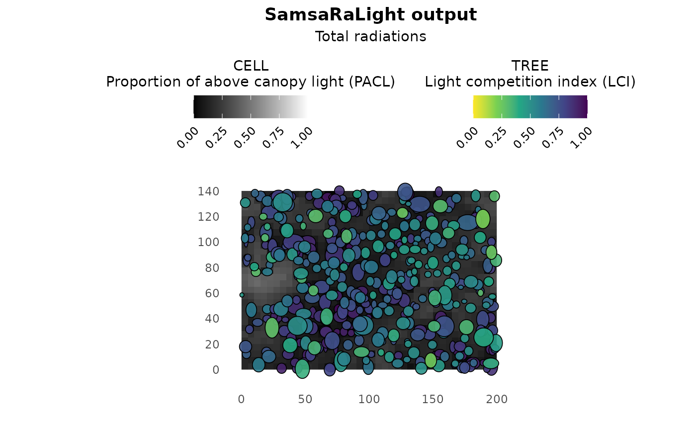
Run SamsaraLight

radiations_bechefa <- SamsaRaLight::get_monthly_radiations(
  latitude = SamsaRaLight::data_bechefa$info$latitude,
  longitude = SamsaRaLight::data_bechefa$info$longitude)

output_bechefa <- SamsaRaLight::run_sl(
  sl_stand = stand_bechefa_filled,
  monthly_radiations = radiations_bechefa
)
#> parallel mode disabled because OpenMP was not available
#> SamsaRaLight simulation was run successfully.

plot(output_bechefa)