4 - Understand ray transmission
Transmission models : porous envelope and turbid medium crowns
Source:vignettes/web_only/4-transmission_interception.Rmd
4-transmission_interception.RmdIntroduction
In previous vignettes, we introduced how to build virtual stands and how to simulate light interception in forest stands. In this tutorial, we focus on a key component of these simulations: the way radiation is attenuated when rays cross tree crowns.
In SamsaRaLight, crown transmission can be modelled using two alternative approaches: a porous envelope model and a turbid medium model. These models differ in their underlying assumptions and in the way crown structure is represented.
The choice of transmission model and its parametrisation directly influences simulated light interception at both the tree and stand levels. Understanding these effects is therefore essential when calibrating the transmission models (see Tutorial 5) and interpreting its outputs.
In this vignette, we first present the two transmission models. We then illustrate their effects using simple virtual stands, first at the tree level and then at the stand level. Finally, we discuss practical implications for parameter selection and calibration.
The transmission models
In SamsaRaLight, crown transmission is controlled by the argument
turbid_medium that is accessible only in the advanced-user
function sl_run_advanced(). Depending on its value, one of
the two following models is used. This parameter is set to
TRUE in the base sl_run() function, thus using
a turbid medium as the default model.
Porous envelope model
When turbid_medium = FALSE, crowns are represented as
semi-transparent envelopes. Each time a ray crosses a crown, its energy
is reduced by a fixed proportion defined by the crown openness. This
parameter is defined by crown_openness column in the tree
inventory and ranges within [0, 1] (not required when using the
sl_run() function).
This approach assumes that: - Crown internal structure is not explicitly represented, - Attenuation is independent of the path length inside the crown, - Transmission is spatially homogeneous within each crown.
As a consequence, the porous envelope model provides a simplified representation of canopy structure. It requires only one intuitive parameter, but it does not account nor for variations in foliage density, neither for the path length of the ray within crowns.
Turbid medium model
When turbid_medium = TRUE, crowns are treated as
homogeneous volumes filled with scattering and absorbing elements. In
this case, light attenuation follows a Beer–Lambert law and depends on
the distance travelled inside the crown.
Attenuation is controlled by the leaf area density LAD with the
mandatory column crown_lad in the tree inventory. Other
parameters controlling the turbid medium model can be tweaked in the
sl_run_advanced() function: the extinction coefficient (by
default fixed at 0.5) and the clumping factor (by default fixed at
1).
This approach explicitly links crown geometry and foliage density to light transmission. Rays travelling longer distances inside dense crowns experience stronger attenuation. The turbid medium model therefore provides a more mechanistic representation of radiative transfer. However, crown LAD value is difficult to calibrate, and thus the default value of 0.5 is commonly used. The tutorial 5 shows a use of virtual sensors to calibrate a site-specific value of LAD.
Tree-level effects of the transmission model
We first investigate how the two transmission models affect light interception at the level of an individual tree. To do so, we create a virtual stand containing a single tree whose diameter ranges from 10 to 100 cm. Crown dimensions are derived from allometric relationships, and several simulations are performed using different LAD and crown openness values.
This experimental design allows us to isolate the effect of crown size and transmission parameters.
Define the stand structure
stand_size_x <- 100
stand_size_y <- 100

trees_inv <- data.frame(
  id_tree = 1,
  species = "Picea abies",
  crown_type = "P", # Paraboloidal crown
  x = stand_size_x / 2,
  y = stand_size_y / 2,
  dbh_cm = seq(10, 200, 1)
)
Estimate crown allometries
To create virtual trees, we use spruce allometric relationships from the Samsara2 model (Courbaud et al. 2015) for estimating crown dimensions based on tree size.
trees_inv <- trees_inv %>%

  # Compute crown dimensions using allometries
  # Taken from Courbaud et al. 2025 for spruce
  dplyr::mutate(

    h_m = exp(3.5300) * exp( - log( exp(3.5300) / 1.3 ) * exp( - 0.0767 * dbh_cm ) ),
    hbase_m = ( 1 / (1 + exp(0.4880)) )  * h_m,

    r_m = exp(-0.774) * ( dbh_cm ^ 0.525 ),
    rs_m = r_m,
    rn_m = r_m,
    re_m = r_m,
    rw_m = r_m,

    volume_m3 = 0.5 * pi * r_m^2 * (h_m - hbase_m) # Volume of a paraboloid
  )
plt_heights <- ggplot(trees_inv %>%
                        dplyr::select(dbh_cm, h_m, hbase_m) %>%
                        tidyr::pivot_longer(c(h_m, hbase_m),
                                            names_to = "var",
                                            values_to = "heights_m"),
                      aes(y = heights_m, x = dbh_cm, linetype = var)) +
  geom_line() +
  theme_bw() +
  theme(legend.position = "none") +
  ylab("h_m (solid) and hbase_m (dotted)")

plt_diameter <- ggplot(trees_inv, aes(y = r_m * 2, x = dbh_cm)) +
  geom_line() +
  theme_bw()

plt_volume <- ggplot(trees_inv, aes(y = volume_m3, x = dbh_cm)) +
  geom_line() +
  theme_bw()

plt_heights | plt_diameter | plt_volume +
  plot_layout()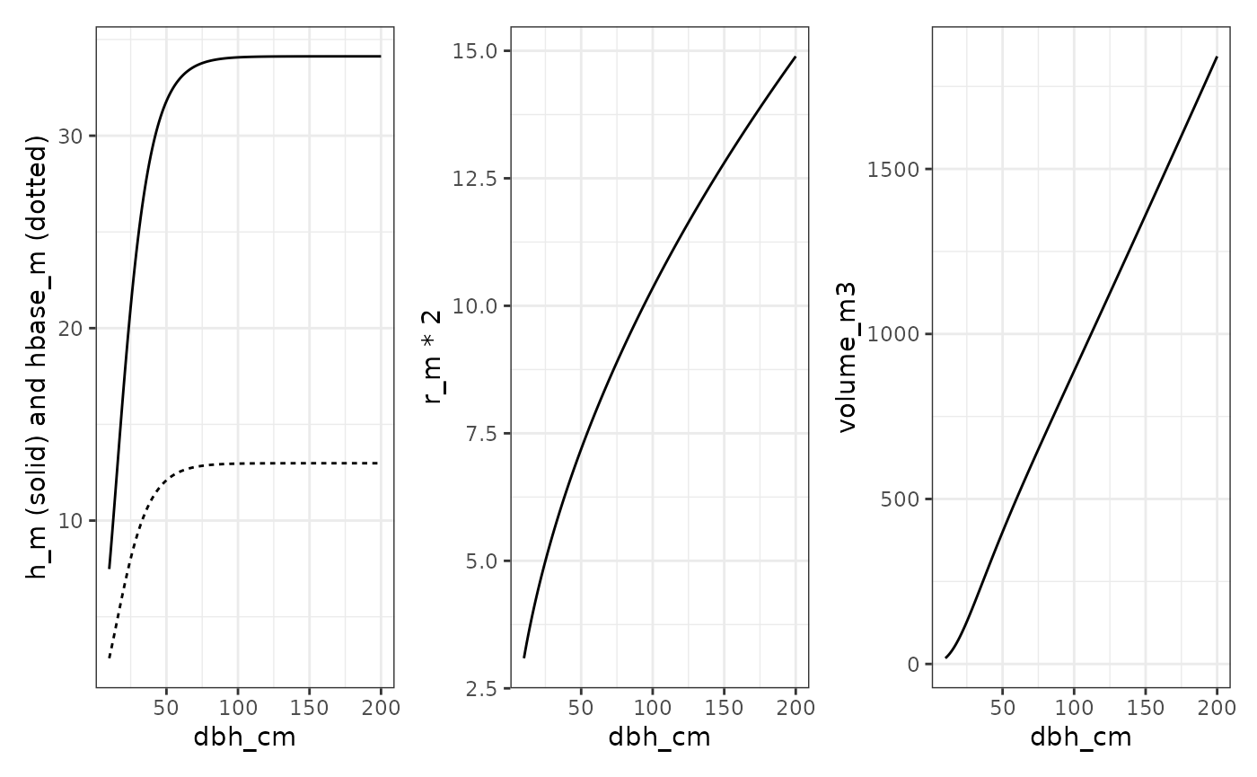
Initialise transmission model parameters
trees_inv_transmit <- dplyr::bind_rows(

  # Tturbid medium model (leaf area density LAD)
  tidyr::crossing(
    trees_inv,
    crown_lad = c(0.05, seq(0.1, 1, by = 0.1), 2:5),
    turbid_medium = TRUE
  ),

  # Prous envelop model (crown openness p)
  tidyr::crossing(
    trees_inv,
    crown_openness = seq(0, 1, by = 0.1),
    turbid_medium = FALSE
  )

) %>%
  dplyr::mutate(
    id_simu = row_number()
  )
Create virtual stands and run SamsaraLight
# Get the monthly radiation data (data_bechefa location)
latitude <- 50.04
longitude <- 5.2

data_rad <- SamsaRaLight::get_monthly_radiations(latitude = latitude, longitude = longitude)

# Initialise the squared inventory zone
core_polygon_df <- data.frame(
  x = c(0, stand_size_x, stand_size_x, 0),
  y = c(0, 0, stand_size_y, stand_size_y)
)
# Here, it is heavy computations, thus load precomputed data that have been created as above
out_trees <- readRDS(
  system.file(
    "extdata",
    "vignette_4_results_trees.rds",
    package = "SamsaRaLight"
  )
)

# ---- PRECOMPUTED DATA SCRIPT ----

# out_trees <- vector("list", length = nrow(trees_inv_transmit))
#
# for (i in trees_inv_transmit$id_simu) {
#
#   print(i)
#
#   # Create the virtual stand
#   tmp_stand <- SamsaRaLight::create_sl_stand(
#     trees_inv_transmit[i,],
#     cell_size = 5,
#     latitude = latitude,
#     slope = 0,
#     aspect = 0,
#     north2x = 90,
#     core_polygon_df = core_polygon_df,
#     verbose = FALSE
#   )
#
#   # Run SamsaraLight
#   tmp_out <- SamsaRaLight::run_sl_advanced(
#     tmp_stand,
#     data_rad,
#     parallel_mode = TRUE,
#     verbose = FALSE,
#
#     # Transmission model and turbid medium parameters
#     turbid_medium = trees_inv_transmit$turbid_medium[i],
#     extinction_coef = 0.5,
#     clumping_factor = 1
#   )
#
#   # Get tree-level output
#   out_trees[[i]] <- tmp_out$output$light$trees
# }
#
# out_trees <- out_trees %>%
#   dplyr::bind_rows(.id = "id_simu") %>%
#   dplyr::mutate(id_simu = as.integer(id_simu))
Transmission within a single crown
The following figures show how intercepted energy varies with crown volume.
plt_trees_lad <- trees_inv_transmit %>%
  dplyr::filter(turbid_medium == TRUE) %>%
  dplyr::left_join(out_trees, by = "id_simu") %>%
  dplyr::mutate(crown_lad = as.factor(crown_lad)) %>%

  ggplot(aes(y = e, x = volume_m3, color = crown_lad)) +
  geom_line() +
  labs(title = "Turbid medium") +
  theme_bw() +
  theme(legend.position = "top",
        plot.title = element_text(hjust = 0.5)) +
  guides(colour = guide_legend(title.position = "top", title.hjust = 0.5))


plt_trees_p <- trees_inv_transmit %>%
  dplyr::filter(turbid_medium == FALSE) %>%
  dplyr::left_join(out_trees, by = "id_simu") %>%
  dplyr::mutate(
    crown_openness =
      factor(crown_openness,
             levels = sort(unique(.$crown_openness), decreasing = TRUE))) %>%

  ggplot(aes(y = e, x = volume_m3, color = crown_openness)) +
  geom_line() +
  labs(title = "Porous envelope") +
  theme_bw() +
  theme(legend.position = "top",
        plot.title = element_text(hjust = 0.5)) +
  guides(colour = guide_legend(title.position = "top", title.hjust = 0.5))


plt_trees_lad | plt_trees_p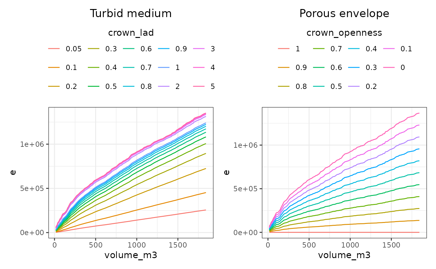
Under the turbid medium model, increasing LAD leads to a progressive decrease in transmitted energy. Because attenuation depends on ray path length, larger crowns are more sensitive to LAD than smaller ones. As a result, the relationship between crown volume and intercepted energy is nonlinear and strongly controlled by LAD. However, the relative effect of LAD decreases as LAD increases. The influence of LAD is strong at low values (approximately between 0.05 and 0.5), moderate between 0.5 and 1, and weak above 1. Beyond this threshold, further increases in LAD have little effect on intercepted light, because light transmission is then mainly controlled by crown dimensions and by whether rays intersect the crown or not.
In the porous envelope model, attenuation is directly controlled by crown openness. For a given openness value, all crowns transmit the same proportion of energy, independently of their internal structure. Consequently, for a given tree size, changes in crown openness induce a constant relative change in light interception, leading to a more linear and predictable response.
Stand-level effect of the transmission model
We now extend the analysis to the stand level, where crowns compete and spatial heterogeneity play a major role.
We generate virtual stands covering a wide range of basal areas and tree densities. For each stand, diameter distributions are reconstructed using Weibull laws, and several transmission parameter values are tested.
This design allows us to analyse how transmission models interact with stand structure.
Define the stand structure
stand_size_x <- 100
stand_size_y <- 100

exp_design <- expand.grid(
  batot_m2ha = 1:40,
  n_trees = seq(100, 400, by = 100)
)
Recreate a virtual diameter distribution
exp_design <- exp_design %>%
  dplyr::mutate(
    param_k = 1.5,
    param_lambda = sqrt( (4 * batot_m2ha) / (pi * n_trees * gamma(1 + 2/param_k)) )
  ) %>%
  dplyr::mutate(
    id_inv = row_number()
  )

trees_inv <- vector("list", length = nrow(exp_design))
for (i in exp_design$id_inv) {

  # Get diameter distribution from Weibull law
  # Parameters are given by the above formula to reach the basal area given a J-shape and the number of trees
  tmp_dbh <- rweibull(exp_design$n_trees[[i]],
                      shape = exp_design$param_k[[i]],
                      scale = exp_design$param_lambda[[i]]) * 100 # from meters in cm

  # Create the trees with a random position
  trees_inv[[i]] <- data.frame(

    id_tree = 1:exp_design$n_trees[[i]],
    dbh_cm = tmp_dbh,
    x = runif(exp_design$n_trees[[i]], 0, stand_size_x),
    y = runif(exp_design$n_trees[[i]], 0, stand_size_y),
    species = "Picea abies"

  ) %>%

    # Estimate crown dimensions
    dplyr::mutate(
      crown_type = "P", # Paraboloidal crown

      h_m = exp(3.5300) * exp( - log( exp(3.5300) / 1.3 ) * exp( - 0.0767 * dbh_cm ) ),
      hbase_m = ( 1 / (1 + exp(0.4880)) )  * h_m,

      r_m = exp(-0.774) * ( dbh_cm ^ 0.525 ),
      rs_m = r_m,
      rn_m = r_m,
      re_m = r_m,
      rw_m = r_m
    )
}

trees_inv <- trees_inv %>%
  dplyr::bind_rows(.id = "id_inv") %>%
  dplyr::mutate(id_inv = as.integer(id_inv))
trees_inv %>%
  dplyr::left_join(exp_design, by = "id_inv") %>%

  dplyr::filter( (n_trees == 100 & batot_m2ha == 10) |
                   (n_trees == 100 & batot_m2ha == 40) |
                   (n_trees == 400 & batot_m2ha == 10) |
                   (n_trees == 400 & batot_m2ha == 40)) %>%
  ggplot(aes(x = dbh_cm,
             linetype = as.factor(n_trees),
             color = as.factor(batot_m2ha))) +
  geom_density() +
  theme_bw()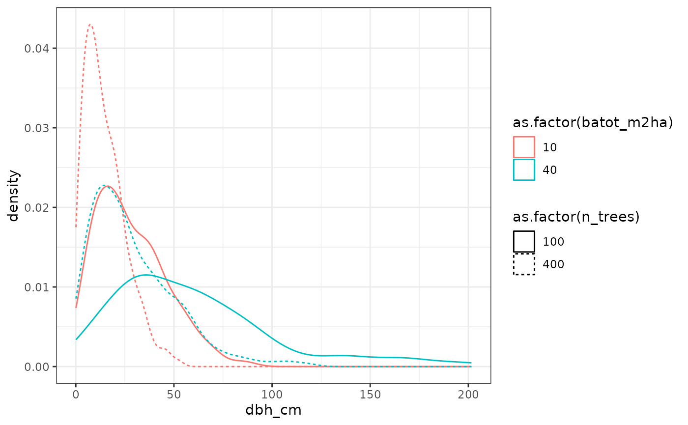
Initialise transmission model parameters
trees_inv_transmit <- dplyr::bind_rows(

  # Turbid medium model (leaf area density LAD)
  tidyr::crossing(
    trees_inv,
    crown_lad = c(0.05, seq(0.1, 1, by = 0.1), 2:5),
    turbid_medium = TRUE
  ),

  # Prous envelop model (crown openness p)
  tidyr::crossing(
    trees_inv,
    crown_openness = seq(0, 1, by = 0.1),
    turbid_medium = FALSE
  )

) %>%
  dplyr::group_by(id_inv, turbid_medium, crown_lad, crown_openness) %>%
  dplyr::mutate(
    id_simu = cur_group_id()
  )
Create virtual stands and run SamsaraLight
# Here, it is heavy computations, thus load precomputed data that have been created as above
out_stands <- readRDS(
  system.file(
    "extdata",
    "vignette_4_results_stands.rds",
    package = "SamsaRaLight"
  )
)

# ---- PRECOMPUTED DATA SCRIPT ----

# id_simus <- unique(trees_inv_transmit$id_simu)
#
# out_stands <- vector("list", length = length(id_simus))
#
# for (i in id_simus) {
#
#   print(i)
#
#   # Get the tre inventory
#   tmp_inv <- trees_inv_transmit %>% dplyr::filter(id_simu == i)
#
#   # Create the virtual stand
#   tmp_stand <- SamsaRaLight::create_sl_stand(
#     tmp_inv,
#     cell_size = 10,
#     latitude = latitude,
#     slope = 0,
#     aspect = 0,
#     north2x = 90,
#     core_polygon_df = core_polygon_df,
#     verbose = FALSE
#   )
#
#   # Run SamsaraLight
#   tmp_out <- SamsaRaLight::run_sl_advanced(
#     tmp_stand,
#     data_rad,
#     parallel_mode = TRUE,
#     verbose = FALSE,
#
#     # Transmission model and turbid medium parameters
#     turbid_medium = unique(tmp_inv$turbid_medium),
#     extinction_coef = 0.5,
#     clumping_factor = 1
#   )
#
#   # Get stand-level output (mean PACL)
#   out_stands[[i]] <- data.frame(
#     id_simu = i,
#     mean_pacl = mean(tmp_out$output$light$cells$pacl)
#   )
# }
#
# out_stands <- out_stands %>%
#   dplyr::bind_rows()
Transmission within the stand
For each simulation, we compute the mean proportion of absorbed canopy light (PACL) at the cell level. Results are then summarised across stands sharing the same structural characteristics.
plt_stands_lad <- trees_inv_transmit %>%
  dplyr::ungroup() %>%
  dplyr::filter(turbid_medium == TRUE) %>%
  dplyr::select(id_simu, id_inv, crown_lad) %>%
  dplyr::distinct() %>%

  dplyr::left_join(exp_design, by = "id_inv") %>%
  dplyr::left_join(out_stands, by = "id_simu") %>%
  dplyr::mutate(crown_lad = as.factor(crown_lad)) %>%

  dplyr::group_by(batot_m2ha, crown_lad) %>%
  dplyr::summarise(mean_pacl.mean = mean(mean_pacl),
                   mean_pacl.lower = quantile(mean_pacl, 0.025),
                   mean_pacl.upper = quantile(mean_pacl, 0.975)) %>%

  ggplot(aes(y = mean_pacl.mean, x = batot_m2ha,
             color = crown_lad, fill = crown_lad)) +
  geom_line() +
  geom_ribbon(aes(ymin = mean_pacl.lower,
                  ymax = mean_pacl.upper),
              alpha = 0.2,
              colour = NA) +

  labs(title = "Turbid medium") +
  theme_bw() +
  theme(legend.position = "top",
        plot.title = element_text(hjust = 0.5)) +
  guides(colour = guide_legend(title.position = "top", title.hjust = 0.5))
#> `summarise()` has regrouped the output.
#> ℹ Summaries were computed grouped by batot_m2ha and crown_lad.
#> ℹ Output is grouped by batot_m2ha.
#> ℹ Use `summarise(.groups = "drop_last")` to silence this message.
#> ℹ Use `summarise(.by = c(batot_m2ha, crown_lad))` for per-operation grouping
#>   (`?dplyr::dplyr_by`) instead.


plt_stands_p <- trees_inv_transmit %>%
  dplyr::ungroup() %>%
  dplyr::filter(turbid_medium == FALSE) %>%
  dplyr::select(id_simu, id_inv, crown_openness) %>%
  dplyr::distinct() %>%

  dplyr::left_join(exp_design, by = "id_inv") %>%
  dplyr::left_join(out_stands, by = "id_simu") %>%
  dplyr::mutate(
    crown_openness =
      factor(crown_openness,
             levels = sort(unique(.$crown_openness), decreasing = TRUE))) %>%

  dplyr::group_by(batot_m2ha, crown_openness) %>%
  dplyr::summarise(mean_pacl.mean = mean(mean_pacl),
                   mean_pacl.lower = quantile(mean_pacl, 0.025),
                   mean_pacl.upper = quantile(mean_pacl, 0.975)) %>%

  ggplot(aes(y = mean_pacl.mean, x = batot_m2ha,
             color = crown_openness, fill = crown_openness)) +
  geom_line() +
  geom_ribbon(aes(ymin = mean_pacl.lower,
                  ymax = mean_pacl.upper),
              alpha = 0.2,
              colour = NA) +

  labs(title = "Porous envelope") +
  theme_bw() +
  theme(legend.position = "top",
        plot.title = element_text(hjust = 0.5)) +
  guides(colour = guide_legend(title.position = "top", title.hjust = 0.5))
#> `summarise()` has regrouped the output.
#> ℹ Summaries were computed grouped by batot_m2ha and crown_openness.
#> ℹ Output is grouped by batot_m2ha.
#> ℹ Use `summarise(.groups = "drop_last")` to silence this message.
#> ℹ Use `summarise(.by = c(batot_m2ha, crown_openness))` for per-operation
#>   grouping (`?dplyr::dplyr_by`) instead.


plt_stands_lad | plt_stands_p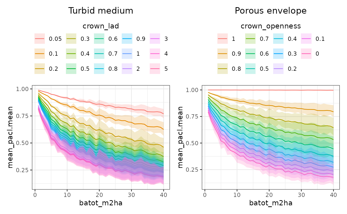
Mean intercepted light first decreases rapidly with increasing total basal area for both transmission models and all tree-level transmission parameters. This initial decline reflects the dominant role of crown presence in controlling ground-level light availability, as increasing stand density rapidly closes canopy gaps and enhances ray interception.
In porous envelope simulations, changes in crown openness produce relatively uniform shifts in light availability. In contrast, in turbid medium simulations, increasing LAD leads to a rapid and strong reduction in below-canopy radiation at low values, followed by a progressive saturation of the LAD effect from about 0.5, reaching a plateau around LAD = 1.
Practical implications for model parametrisation
These results highlight that transmission parameters cannot be selected independently of the chosen model and must therefore be carefully calibrated together. In practice, we commonly use the turbid medium approach, as it better reflects ontogenetic effects on light attenuation by accounting for both the ray path length within crowns—which increases with tree size—and the internal leaf distribution controlled by tree-level LAD.
However, LAD calibration is a major gap in literature, and is commonly fixed at 0.5m2/m3. In practice, LAD calibration should rely on independent measurements, such as hemispherical photographs or ground-based radiation sensors. Virtual sensor approaches, as illustrated in the next tutorial, can support this calibration process.