Non-rectangular inventory zone

library(SamsaRaLight)
library(dplyr)
#> 
#> Attaching package: 'dplyr'
#> The following objects are masked from 'package:stats':
#> 
#>     filter, lag
#> The following objects are masked from 'package:base':
#> 
#>     intersect, setdiff, setequal, union

Introduction

In previous tutorials, inventories were assumed to be simple, axis-aligned rectangles. In practice, however, forest inventories are often more complex, and may not be necessary rectangle depending on the inventory protocol.

In this vignette, we illustrate the case of an non-rectangular inventory. The sampled area is defined by an irregular polygon (e.g. a combination of circular plots), filled around by virtual trees.

Context and data

We now consider the example inventory Cloture20, stored in the package as SamsaRaLight::data_cloture20.

This inventory was collected by Gauthier Ligot in Wallonia, Belgium, as part of the CLOTURE project, which investigates the effect of fences on beech and oak plots with varying beech proportions. In this case, the plot is primarily made up of beech trees (Fagus sylvatica). The crowns are described with full asymmetric shapes “8E”. The inventory protocol is complex and resulted in non-rectangular inventory zones formed from multiple circular areas. Thus, the core polygon is defined by 94 vertices:

str(SamsaRaLight::data_cloture20$core_polygon)
#> 'data.frame':    94 obs. of  2 variables:
#>  $ x: num  54 56.4 59.1 61.9 64.8 ...
#>  $ y: num  70.4 72.2 73.6 74.6 75.2 ...

Virtual stand with complex core polygon

First, we can create the virtual stand by setting the pre-defined core polygon stored in the package. Representing the inventory as a rectangle in this case would be inconsistent with the field protocol. Therefore, the polygon is preserved inside a larger virtual stand with modify_polygon = "none" and the virtual stand is filled around the inventory zone with fill_around = TRUE.

stand_cloture_filled <- SamsaRaLight::create_sl_stand(
  trees_inv = SamsaRaLight::data_cloture20$trees,
  cell_size = 5,
  
  latitude = SamsaRaLight::data_cloture20$info$latitude,
  slope    = SamsaRaLight::data_cloture20$info$slope,
  aspect  = SamsaRaLight::data_cloture20$info$aspect,
  north2x = SamsaRaLight::data_cloture20$info$north2x,
  
  core_polygon_df = SamsaRaLight::data_cloture20$core_polygon,
  modify_polygon = "none",
  fill_around = TRUE
)
#> SamsaRaLight stand successfully created.

plot(stand_cloture_filled)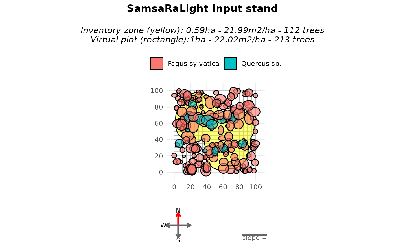

summary(stand_cloture_filled)
#> 
#> SamsaRaLight stand summary
#> ================================
#> 
#> 
#> Inventory (core polygon):
#>   Area              : 0.59 ha
#>   Trees             : 112
#>   Density           : 190.5 trees/ha
#>   Basal area        : 21.99 m2/ha
#>   Quadratic mean DBH: 38.3 cm
#> 
#> Simulation stand (core + filled buffer):
#>   Area              : 1.00 ha
#>   Trees             : 213
#>   Density           : 213.0 trees/ha
#>   Basal area        : 22.02 m2/ha
#>   Quadratic mean DBH: 36.3 cm
#> 
#> Stand geometry:
#>   Grid              : 20 x 20 (400 cells)
#>   Cell size         : 5.00 m
#>   Slope             : 0.00 deg
#>   Aspect            : 0.00 deg
#>   North to X-axis   : 90.00 deg
#> 
#> Number of sensors: 0

Run SamsaraLight

Finally, the radiation data and the simulation run are done as usual:

data_radiations_cloture <- SamsaRaLight::get_monthly_radiations(
  latitude  = SamsaRaLight::data_cloture20$info$latitude,
  longitude = SamsaRaLight::data_cloture20$info$longitude
)

output_cloture_filled <- SamsaRaLight::run_sl(
  sl_stand = stand_cloture_filled,
  monthly_radiations = data_radiations_cloture
)
#> parallel mode disabled because OpenMP was not available
#> SamsaRaLight simulation was run successfully.

plot(output_cloture_filled)

summary(output_cloture_filled)
#> 
#> SamsaRaLight simulation summary
#> ================================
#> 
#> Trees (crown interception)
#> ---------------------------
#>       epot               e                 lci        
#>  Min.   :  30904   Min.   :   694.8   Min.   :0.0906  
#>  1st Qu.: 139463   1st Qu.: 14399.6   1st Qu.:0.5837  
#>  Median : 244016   Median : 43603.7   Median :0.7845  
#>  Mean   : 391760   Mean   :148149.6   Mean   :0.7233  
#>  3rd Qu.: 617430   3rd Qu.:273832.3   3rd Qu.:0.8966  
#>  Max.   :1319122   Max.   :815029.7   Max.   :0.9899  
#> 
#> Cells (ground light)
#> -------------------
#>        e                pacl             punobs      
#>  Min.   :  91.59   Min.   :0.02434   Min.   :0.0000  
#>  1st Qu.: 356.87   1st Qu.:0.09485   1st Qu.:0.5240  
#>  Median : 566.30   Median :0.15051   Median :0.6896  
#>  Mean   : 606.90   Mean   :0.16130   Mean   :0.6293  
#>  3rd Qu.: 843.78   3rd Qu.:0.22426   3rd Qu.:0.7710  
#>  Max.   :1532.63   Max.   :0.40734   Max.   :0.8858  
#> 
#> Sensors
#> -------
#> No sensor energy variables available